
Reading Propagation Maps
How to interpret sector rays, frequency-dependent attenuation, coverage evidence, and the current map layers.
A.T.O.M visualizes deterministic RF planning estimates across frequency bands using Ankara's urban topology. The images are model outputs, not measured coverage maps.
4G LTE Coverage (2.6 GHz)
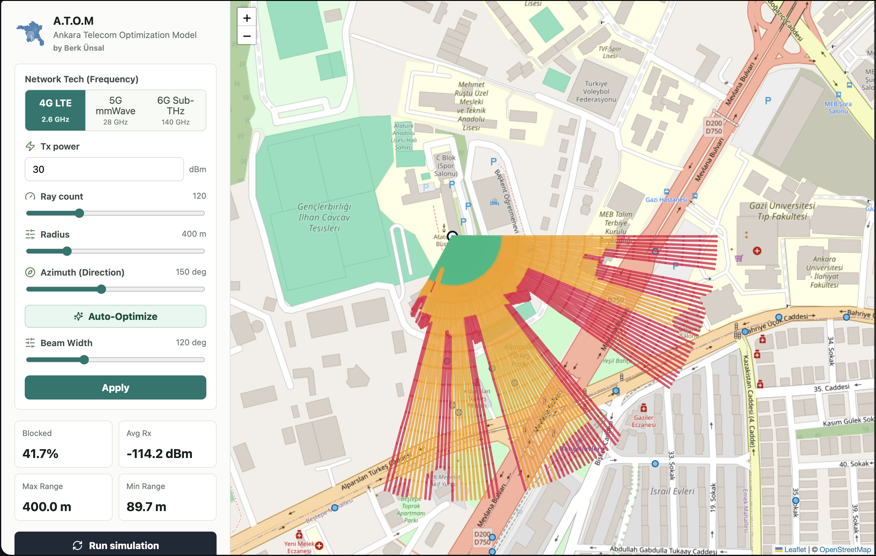
Characteristics
- Wavelength: 11.5 cm
- Coverage Type: Wide-area with building penetration
- Penetration Loss: roughly +8 dB per wall crossing in the current LTE model
- Urban Canyon Effect: Moderate (signals reach side streets)
Interpretation
The 4G simulation shows:
- 🟢 Green zones: Strong indoor coverage (-50 to -70 dBm)
- 🟡 Yellow zones: Moderate coverage (-70 to -90 dBm), usable for typical applications
- 🔴 Red zones: Marginal coverage (-90 to -110 dBm), possible dead zones
Key Insight: Lower FSPL and the model's lower per-wall loss generally let 4G estimates extend farther than higher-frequency modes.
5G mmWave Coverage (28 GHz)
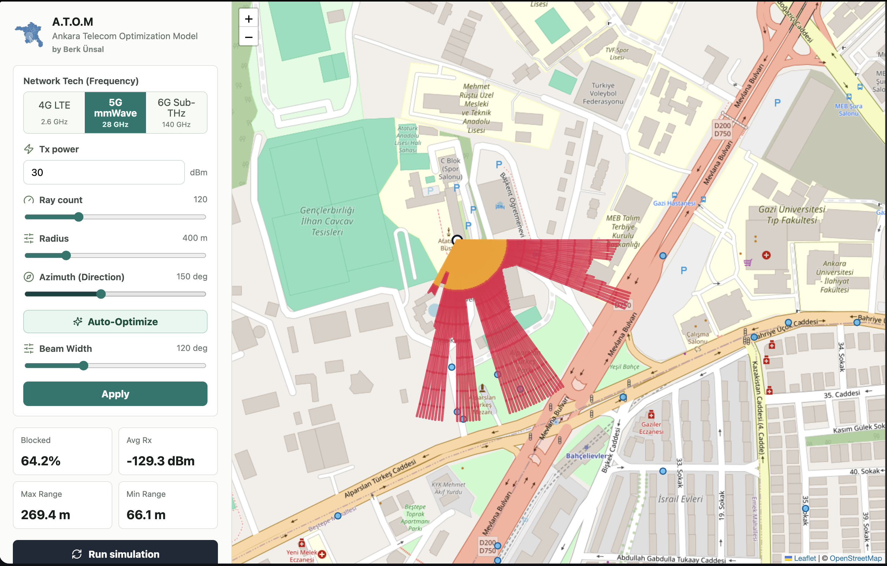
Characteristics
- Wavelength: 1.07 cm
- Coverage Type: Directional, urban-specific hotspots
- Penetration Loss: roughly +30 dB per wall crossing in the current mmWave model
- Line-of-Sight Requirement: Often necessary for usable signal
Interpretation
The 5G visualization reveals:
- 🟢 Green zones: Excellent LOS coverage on main avenues
- 🟡 Yellow zones: Partial coverage after distance and wall-loss attenuation
- 🔴 Red zones: Deep urban canyons blocked by building walls
Key Insight: 5G requires careful site placement to reach street-level users. Antenna orientation (azimuth) dramatically affects coverage.
6G Research Profile Coverage (140 GHz)
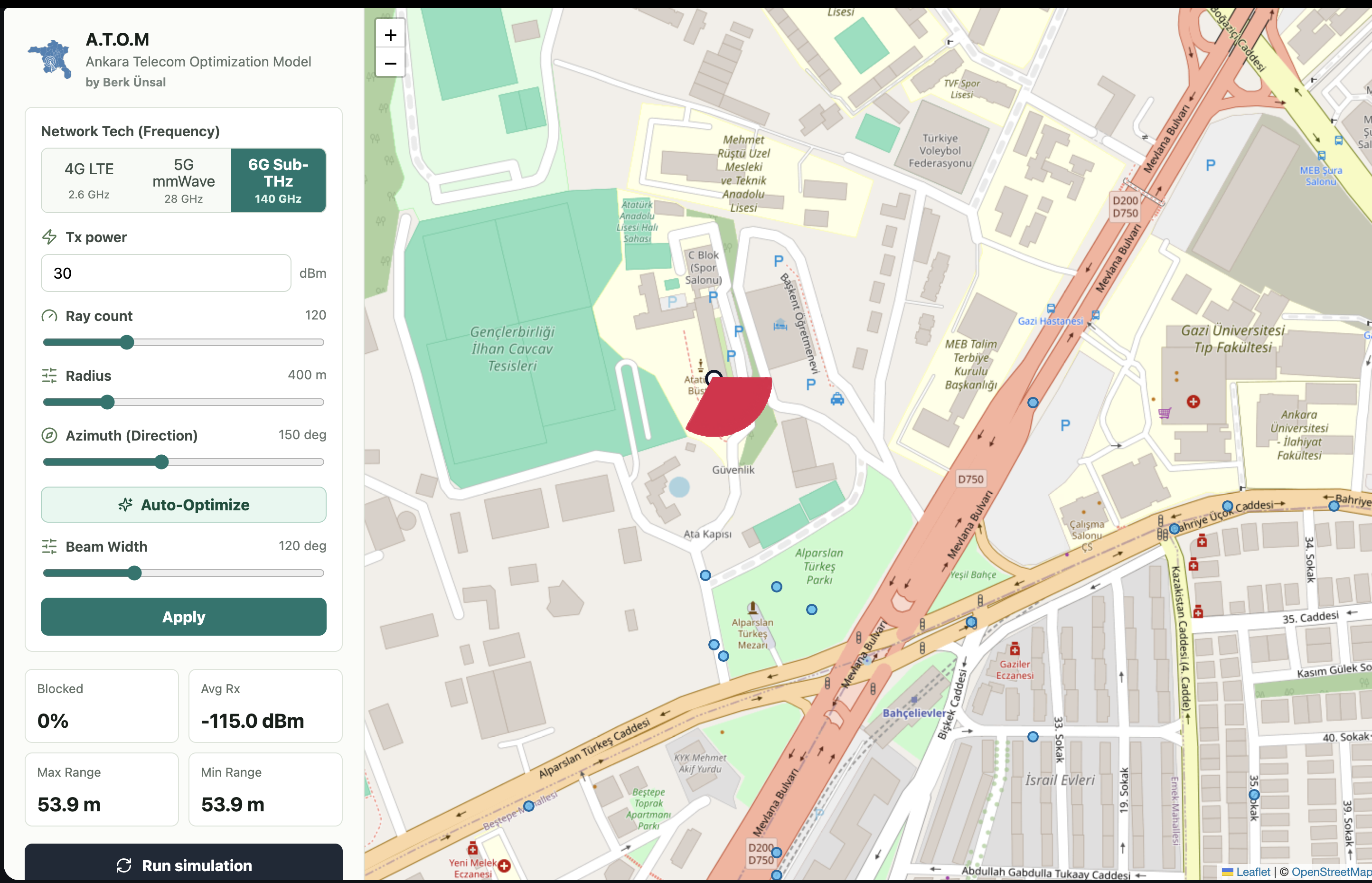
Characteristics
- Wavelength: 2.14 mm (near-optical)
- Coverage Type: Ultra-localized comparative planning overlay
- Penetration Loss: roughly +80 dB per wall crossing in the current Sub-THz model
- Line-of-Sight Requirement: Mandatory for coverage
Interpretation
The 6G heatmap demonstrates:
- 🟢 Green zones: Only direct line-of-sight points
- 🟡 Yellow zones: Minimal; mostly absent
- 🔴 Red zones: Vast majority (blocked by buildings)
Key Insight: The 140 GHz mode is a 6G research profile, not a standardized network-quality model. Its short-range result is useful for comparative planning and is not a deployment guarantee.
Auto-Optimized 5G Sector
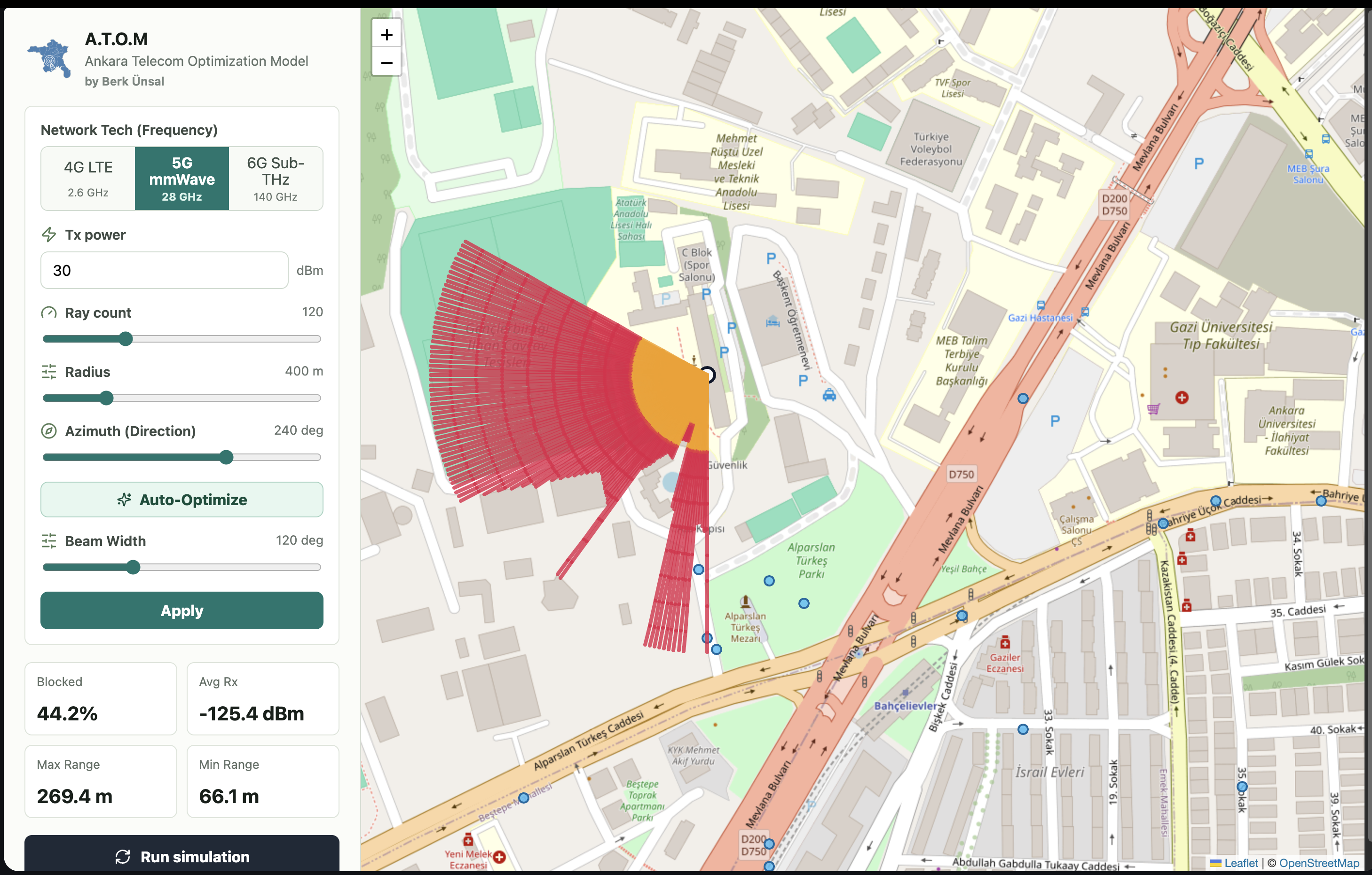
Algorithm Result
This simulation shows the optimal antenna azimuth computed by A.T.O.M's sweep-and-score algorithm:
- Demand-aware score: POI demand, residential-density demand, and capped coverage tie-breakers guide azimuth selection
- Beam Width: 65° (typical 3-sector configuration)
- Optimization Runtime: ~250 ms
Interpretation
The auto-optimized placement achieves:
- ✅ Stronger demand-serving direction within distance constraints
- Stronger modeled coverage toward demand-weighted locations
- A reproducible azimuth recommendation from the configured sweep
Key Insight: The optimizer consistently compares candidate azimuths using the same demand and coverage score. It does not predict live-network spectral efficiency.
Color Mapping Reference
The map uses a display-only received-power palette. It is not a
universal service-quality legend: receiver sensitivity is per effective
cell, building service uses a separate -100 dBm threshold,
and interference serviceability uses RSRP/SINR/RSRQ thresholds.
| Color | Signal Range | Quality | Use Case |
|---|---|---|---|
| 🟢 Green | -50 to -70 dBm | Excellent | Voice, video, IoT |
| 🟡 Yellow | -70 to -90 dBm | Good | Voice, messaging |
| 🔴 Red | -90 to -110 dBm | Poor | Emergency services |
| ⚫ Black | Below the configured display floor | Visually suppressed | Presentation only; raw values remain in the API |
Comparative Analysis: 4G vs 5G vs 6G
Coverage Radius Comparison
| Technology | Typical Radius | Max Radius |
|---|---|---|
| 4G | 2 km (urban) | 5 km (rural) |
| 5G mmWave | 300 m planning preset | 1 km configurable limit |
| 6G research profile | 50 m (illustrative) | 200 m (illustrative planning bound) |
Site Density Required
| Technology | Sites per km² | Building Density Impact |
|---|---|---|
| 4G | 1-3 | Low (penetrates walls) |
| 5G mmWave | 10-50 | High (requires LOS) |
| 6G research profile | 100+ | Very High (illustrative street-level comparison) |
Urban Canyon Effect
The visualizations clearly show how building density impacts each band:
- 4G: Usually produces the broadest modeled reach because FSPL and wall loss are lower.
- 5G: Produces more localized, directional modeled coverage at 28 GHz.
- 6G: Is a research profile with the strongest configured wall attenuation and shortest illustrative planning range.
Understanding the Heatmaps
Ray Segments
Each heatmap consists of thousands of ray segments (colored lines):
- Start Point: Transmitter antenna
- End Point: Coverage measurement location (typically 20-100 meters away)
- Color: Represents signal strength at that distance/direction
- Direction: Shows propagation pattern and antenna beam orientation
Reading the Visualization
- Green Zones: Primary coverage area; reliable service expected
- Yellow Zones: Secondary coverage; service possible with optimal conditions
- Red Zones: Marginal; not recommended for primary coverage
- No Color: Below the visual display floor or outside the rendered evidence; this does not mean the API value is NoData or that it fails every serviceability rule
Analytical Surface Layer
The Signal surface tool replaces dense point markers with a regular raw single-cell received-power raster drawn below operational markers. Adjust opacity to compare it with the basemap and select a display floor to hide weaker cells; that floor is visual only. Valid below-sensitivity values remain in the surface, while NoData means radius/beam geometry exclusion. Contours are unsmoothed marching-square line segments at the selected dBm thresholds; they are deterministic grid evidence, not kriged measurement isolines. The surface is calculated for one selected cell, so it is not an aggregate network-coverage claim.
RF Map Display Controls
The compact RF control group keeps the two evidence types independent:
- Signal toggles the received-power surface when one has been generated.
- Rays toggles the segmented propagation paths without issuing another RF request.
- All cells, Selected cell, and Hidden control which network ray paths are rendered. The Selected cell choice uses the separate Focus cell selector; it does not change the Pareto solution selected in Results.
Until a surface is generated, rays are the visible RF fallback. Generating a received-power surface switches the map to a surface-first view and hides rays; rays can be enabled again for diagnostic inspection. Presentation-only changes are local browser state. RF settings, cell selection, or a new optimization/evaluation clear incompatible rendered evidence and require the normal explicit analysis action.
The raster uses the fast sector FSPL/antenna/wall model. It does not inherit optional terrain, gas, rain, vegetation, or diffraction settings from a point-to-point profile.
Enable Viewport buildings in Layers at zoom 12 or closer to request only the visible building footprints. Fill hue reflects normalized material when known and opacity increases modestly with inferred height; it is contextual geometry, not a surveyed 3D mesh.
Vertical Path Profile
The Propagation tool's path view shows ground, building tops, endpoint elevations, the direct LOS line, 60% Fresnel clearance, and any dominant obstruction. The adjacent component table is the authoritative explanation of which optional losses were enabled. A red obstruction does not imply a complete multiple-edge diffraction or reflected-path solution.
Interactive Exploration
In the web interface, you can:
- 🔄 Adjust antenna azimuth and watch coverage rotate
- 📊 Switch between frequency bands and compare
- 🧭 Focus a selected network cell while keeping the planning selection unchanged
- 🗺️ Switch between the received-power surface and diagnostic ray evidence
- 🎯 Toggle beamforming on/off to see impact
- 📍 Click points to see exact signal strength (Rx dBm)
Validation Boundary
A.T.O.M has not been calibrated against operator drive tests or UE measurements. Treat Rx, RSRP, SINR, and RSRQ values as planning estimates for scenario comparison, then validate deployment decisions with calibrated tools and field measurements.
Export and Integration
Analytical surfaces can be exported as float32 EPSG:4326 GeoTIFF, contour GeoJSON, or grid-center CSV. Viewport building queries return GeoJSON or CSV/WKT. These can be used in:
- 🗺️ ArcGIS: Professional GIS analysis
- 🌍 Google Earth: 3D visualization
- 📋 QGIS: Open-source mapping
- 🔗 Custom applications: Any GeoJSON-compatible tool
Next: Learn the physics behind these visualizations in Algorithms & Physics.